Hands-on: CwCF using Deep-RL

Classification with Costly Features (CwCF)

This article presents a practical use of Deep-RL in a problem I’ve been working on. It shows some decisions and complications that may arise in real-world domains. So, if you’re interested, let’s get started.

In many domains, you have a sense of cost - it can come in the form of money, time, performance, discomfort and many others. I actually started investigating this problem with a real-world problem in computer security. In a company a partly worked for, they develop machine-learning algorithms to analyze network flows to detect systems infected with malware. Such a system usually displays an abnormal activity. In this setting, features are computed from raw packets captured from the network communication and then they are processed by several layers of machine learning algorithms, ordered from fastest to more profound, and at each time they select only a tiny portion of the data to be processed further. In the end, there are only a handful of cases, which need to be examined with a human operator, who usually queries different cloud services (such as VirusTotal) to analyze the data.

But this latest piece of the chain is the weakest point - the goal would be to replace the human operator with a machine-learned algorithm that can query the cloud services and make a good prediction. Here, the cloud service usually limits the queries, so we have to learn how to use these scarce resources.

As the problem is naturally sequential, RL immediately comes to mind as a suitable tool. The agent would ask for different resources, learn information and finally make a prediction, both maximizing accuracy and minimizing the cost, as in the picture below:

Here, at each step the agent requests a feature and decides what to do next. Either he selects another feature, or it can classify. The important fact is that it always uses all the information it has acquired so far for the decision.

Formal description

Let’s simplify the problem first. Let’s assume that the sample (e.g., the computer on the network) is just a vector of real numbers \(x \in \mathbf{R}^n\), and each of the features has a cost, that has to be paid when revealing it. Then we have a model, which we consists of two functions: The function \(y_\theta(x)\) returns the predicted class and \(z_\theta(x)\) returns the total cost for that prediction. The goal is then to learn the model \(\theta\), such that we minimize the loss \(\ell\) (e.g., binary loss - 0 if classification is correct, 1 if not) and total cost, averaged over whole training dataset:

With \(\lambda\) we can force the focus more to the classification error or the cost, it is a trade-off parameter. The problem with the formula is that it is not differentiable, so we can’t minimize it with gradient descent. But what we can do is to create an environment, where at each step the agent can ask for one feature which has not yet been revealed, or classify with one of the classes. If we say that \(c_{f_i}\) is the cost for feature \(i\), then the reward for the feature-selecting actions would be \(-\lambda c_{f_i}\) and the reward for the classification action \(-\ell(\hat y, y)\), as shown below:

In such a defined environment, we can see that the total reward the agent would receive per episode is:

That is exactly what we want! In RL, we are trying to maximize the expected reward and here it is equal to minimizing the defined objective above. If we solved this environment precisely, we would obtain the optimal solution.

Deep Reinforcement Learning

However, since the input space is continuous and high-dimensional, precise computation is out of the question. Here comes the Deep-RL which should help us to solve this problem. Should we use Q-learning or Policy Gradient methods? Actually, both should work and I chose Q-learning.

There are a few things to think about. First, how should we encode the current sample for the neural network? More specifically, what should we do with the features we don’t know? The natural answer is to substitute them with a mean, and because we are normalizing our dataset (which is nearly always a good thing), the mean corresponds to zero. But now we have another problem - how can the network distinguish between the two meanings of zero - a feature is missing, or that feature is actually a zero. A simple solution is to augment the input with another vector which contains 1 if the feature is present and 0 if not.

The model shouldn’t be able to ask for the same feature multiple times. Again, the solution is simple - just ignore the outputs for the actions that aren’t available. That is, when we are selecting the best action, we count only those which are available and also we ignore the unavailable actions during the Q function updates.

When everything is set, it is only a matter of using DQN as a tool to find an approximate solution. Well, almost - currently RL requires a large amount of tinkering, experimenting and lot of effort to make it work. As Alex Irpan said in his blog, RL can fail in many ways. One good example is that I had to use very large batches (about 50 000 steps in one batch) to make this algorithm work, which is very different from what original DQN used. But that should not prevent you from trying!

Results

The method performs much better compared to competing algorithms, although they were specifically designed for this problem. In light of this, let’s take a lesson - the time may be right to prefer a general solution over a specific one.

I will highlight only one particular result in the MNIST number recognition dataset. For full comparison with other algorithm and more datasets, I refer you to the paper. I treat each separate pixel as one feature, resulting in \(28 \times 28=784\) features. MNIST dataset, however, does not have any costs associated, hence I treat them with equal importance.

Below is a performance graph, with an average number of selected features on the x axis, and accuracy on y axis. Here I want to highlight, that a plain neural-network based classifier (with a comparable number of parameters) achieves 97.7% accuracy (see the black line). But that’s when it sees all 784 pixels. The RL model achieves 95% accuracy looking only at 50 pixels on average!

Let’s analyze it further, what pixels does it look at? First, I averaged all instances of each class (i.e., to determine how an average zero looks like), and then also averaged over all features taken in different instances for each class. Below you see a heatmap of what pixels are probed:

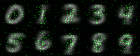
To me, it seems that the model tries to probe areas which are specific to certain digits. I.e., in case of zero, it probes the center, which is black, and then few pixels around to make sure that is indeed zero.

Let’s look at the model from another angle: How many features it requires across different samples? Below you can see a histogram, where on x axis there is the number of features requested and on the y axis shows how often that occured.

You can see that most samples are classifier with about 20-100 features. Further examination revealed that the model indeed treats different samples differently, asking only for features which are important in the particular case. In MNIST dataset, there seem to be only samples with similar classification difficulty. But in other datasets, I often see multiple modes in the histogram, which may reveal something about the dataset itself. I.e., there may be several groups of samples, some of which can be classified immediately, some with a few features and some which are really hard.

Conclusion

I tried to describe a problem where RL can be practically used. The main message is that RL may be mature enough for it to be used as a practical tool. And maybe you should try first before implementing a problem-specific solution, if your domain allows it. If you’re interested in more details about the CwCF problem and the RL solution, you can download the paper, slides, poster or examine the code. If you want to cite this work, please use the following:

@inproceedings{janisch2019classification,
  title={Classification with Costly Features using Deep Reinforcement Learning},
  author={Janisch, Jaromír and Pevný, Tomáš and Lisý, Viliam},
  booktitle={AAAI Conference on Artificial Intelligence},
  year={2019}
}