This article is part of series Let’s make a DQN.
Introduction
Last time we tried to get a grasp of necessary knowledge and today we will use it to build an Q-network based agent, that will solve a cart pole balancing problem, in less than 200 lines of code.
The complete code is available at github.
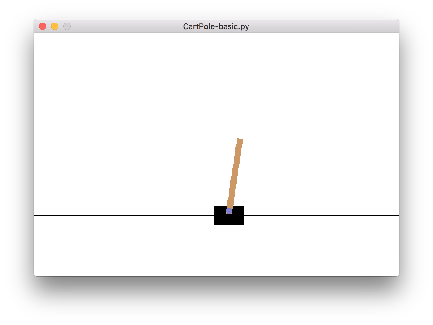
The problem looks like this:

There’s a cart (represented by the black box) with attached pole, that can rotate around one axis. The cart can only go left or right and the goal is to balance the pole as long as possible.
The state is described by four values - cart position, its velocity, pole angle and its angular velocity. At each time step, the agent has to decide whether to push the cart left or right.
If the pole is up, above a certain angle, the agent receives a reward of one. If it falls below this critical angle, the episode ends.
The important fact here is that the agent does not know any of this and has to use its experience to find a viable way to solve this problem. The algorithm is just given four numbers and has to correlate them with the two available actions to acquire as much reward as possible.
Prerequisites
Our algorithm won’t be resource demanding, you can use any recent computer with Python 3 installed to reproduce results in this article. There are some libraries that you have to get before we start. You can install them easily with pip command:
pip install theano keras gym
This will fetch and install Theano, a low level library for building artificial neural networks. But we won’t use it directly, instead we will use Keras as an abstraction layer. It will allow us to define our ANN in a compact way. The command also installs OpenAI Gym toolkit, which will provide us with easy to use environments for our agent.
The Keras library uses by default TensorFlow, which is a different library from Theano. To switch to Theano, edit ~/.keras/keras.json file so it contains this line:
"backend": "theano",
Implementation
Before we jump on to the code itself, let’s think about our problem in an abstract way. There’s an agent, which interacts with the environment through actions and observations. The environment reacts to agent’s actions and supply information about itself. The agent will store the encountered experience in its memory and use its (artificial) intelligence to decide what actions to take. The next diagram shows an abstraction of the problem:

Following our intuition, we will implement four classes - Environment, Agent, Brain and Memory, with these methods:
Environment
    run()         # runs one episode

Agent
    act(s)        # decides what action to take in state s
    observe(sample) # adds sample (s, a, r, s_) to memory
    replay()    # replays memories and improves

Brain
    predict(s)    # predicts the Q function values in state s
    train(batch)  # performs supervised training step with batch

Memory
    add(sample)     # adds sample to memory
    sample(n)   # returns random batch of n samples
With this picture in mind, let’s look at each of these in more detail.
Environment
The Environment class is our abstraction for OpenAI Gym. Its only method run() handles one episode of the problem. Look at an excerpt from the run() function:
s = env.reset()
while True:
    a = agent.act(s)
    s_, r, done, info = env.step(a)

  if done:
        s_ = None

    agent.observe( (s, a, r, s_) )
    agent.replay()

    s = s_

  if done:
        break
In the main loop, the agent decides what action to take, based on given state. The environment then performs this action and returns a new state and a reward.
We will mark the end of the episode by setting the new state s_ to None. The actual state is not needed because there is one terminal state.
Then the agent observes the new sample (s, a, r, s’) and performs a learning step.
Brain
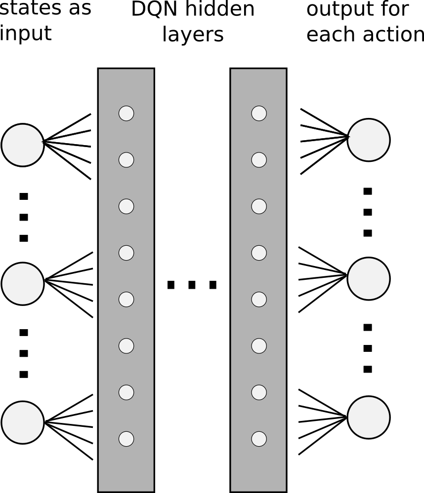
The Brain class encapsulates the neural network. Our problem is simple enough so we will use only one hidden layer of 64 neurons, with ReLU activation function. The final layer will consist of only two neurons, one for each available action. Their activation function will be linear. Remember that we are trying to approximate the Q function, which in essence can be of any real value. Therefore we can’t restrict the output from the network and the linear activation works well.
Instead of simple gradient descend, we will use a more sophisticated algorithm RMSprop, and Mean Squared Error (mse) loss function.
Keras library allows us to define such network surprisingly easily:
    model = Sequential()

    model.add(Dense(output_dim=64, activation='relu', input_dim=stateCount))
    model.add(Dense(output_dim=actionCount, activation='linear'))

    opt = RMSprop(lr=0.00025)
    model.compile(loss='mse', optimizer=opt)
The train(x, y) function will perform a gradient descend step with given batch.
    def train(self, x, y):
        model.fit(x, y, batch_size=64)
Finally, the predict(s) method returns an array of predictions of the Q function in given states. It’s easy enough again with Keras:
    def predict(self, s):
        model.predict(s)
Memory
The purpose of the Memory class is to store experience. It almost feels superfluous in the current problem, but we will implement it anyway. It is a good abstraction for the experience replay part and will allow us to easily upgrade it to more sophisticated algorithms later on.
The add(sample) method stores the experience into the internal array, making sure that it does not exceed its capacity. The other method sample(n) returns n random samples from the memory.
Agent
Finally, the Agent class acts as a container for the agent related properties and methods. The act(s) method implements the ε-greedy policy. With probability epsilon, it chooses a random action, otherwise it selects the best action the current ANN returns.
    def act(self, s):
        if random.random() < self.epsilon:
            return random.randint(0, self.actionCnt-1)
        else:
            return numpy.argmax(self.brain.predictOne(s))
We decrease the epsilon parameter with time, according to a formula:
\[\varepsilon = \varepsilon_{min} + (\varepsilon_{max} - \varepsilon_{min}) e^{-\lambda t}\]The λ parameter controls the speed of decay. This way we start with a policy that explores greatly and behaves more and more greedily over time.
The observe(sample) method simply adds a sample to the agent’s memory.
    def observe(self, sample):  # in (s, a, r, s_) format
        self.memory.add(sample)
The last replay() method is the most complicated part. Let’s recall, how the update formula looks like:
\[Q(s, a) \xrightarrow{} r + \gamma \max_a Q(s', a)\]This formula means that for a sample (s, r, a, s’) we will update the network’s weights so that its output is closer to the target.
But when we recall our network architecture, we see, that it has multiple outputs, one for each action.

We therefore have to supply a target for each of the outputs. But we want to adjust the ouptut of the network for only the one action which is part of the sample. For the other actions, we want the output to stay the same. So, the solution is simply to pass the current values as targets, which we can get by a single forward propagation.
Also, we have a special case of the episode terminal state. Remember that we set a state to None in the Environment class when the episode ended. Because of that, we can now identify such a state and act accordingly.
When the episode ends, there are no more states after and so our update formula reduces to
\[Q(s, a) \xrightarrow{} r\]In this case, we will set our target only to r.
Let’s look at the code now. First we fetch a batch of samples from the memory.
batch = self.memory.sample(BATCH_SIZE)
We can now make the predictions for all starting and ending states in our batch in one step. The underlaying Theano library will parallelize our code seamlessly, if we supply an array of states to predict. This results to a great speedup.
    no_state = numpy.zeros(self.stateCnt)

    states = numpy.array([ o[0] for o in batch ])
    states_ = numpy.array([ (no_state if o[3] is None else o[3]) for o in batch ])

    p = agent.brain.predict(states)
    p_ = agent.brain.predict(states_)
Notice the no_state variable. We use it as a dummy replacement state for the occasions where the final state is None. The Theano librarary cannot make a preditiction for a None state, therefore we just supply an array full of zeroes.
The p variable now holds predictions for the starting states for each sample and will be used as a default target in the learning. Only the one action passed in the sample will have the actual target of \(r + \gamma \max_a Q(s', a)\).
The other p_ variable is filled with predictions for the final states and is used in the \(\max_a Q(s', a)\) part of the formula.
We now iterate over all the samples and set proper targets for each sample:
    for i in range(batchLen):
        o = batch[i]
        s = o[0]; a = o[1]; r = o[2]; s_ = o[3]

        t = p[i]
        if s_ is None:
            t[a] = r
        else:
            t[a] = r + GAMMA * numpy.amax(p_[i])

        x[i] = s
        y[i] = t
Finally, we call our brain.train() method:
self.brain.train(x, y)
Main
To make our program more general, we won’t hardcode state space dimensions nor number of possible actions. Instead we retrieve them from the environment. In the main loop, we just run the episodes forever, until the user terminates with CTRL+C.
PROBLEM = 'CartPole-v0'
env = Environment(PROBLEM)

stateCnt  = env.env.observation_space.shape[0]
actionCnt = env.env.action_space.n

agent = Agent(stateCnt, actionCnt)

while True:
    env.run(agent)
Normalization
Although a neural network can in essence adapt to any input, normalizing it will typically help. We can sample a few examples of different states to see what they look like:
[-0.0048  0.0332 -0.0312  0.0339]
[-0.01   -0.7328  0.0186  1.1228]
[-0.166  -0.4119  0.1725  0.8208]
[-0.0321  0.0445  0.0284 -0.0034]
We see that they are essentially similar in their range, and their magnitude do not differ substantially. Because of that, we won’t normalize the input in this problem.
Hyperparameters
So far we talked about the components in a very generic way. We didn’t give any concrete values for the parameters mentioned in previous sections, except for the neural network architecture. Following parameters were chosen to work well in this problem:
| Parameter | Value |
|---|---|
| memory capacity | 100000 |
| batch size | 64 |
| γ | 0.99 |
| εmax | 1.00 |
| εmin | 0.01 |
| λ | 0.001 |
| RMSprop learning rate | 0.00025 |
Results
You can now download the full code and try it for yourself: https://github.com/jaromiru/AI-blog/blob/master/CartPole-basic.py
It’s remarkable that with less than 200 lines of code, we can implement a Q-network based agent. Although we used CartPole-v0 environment as an example, we can use the same code for many different environments, with only small adjustments. Also, our agent runs surprisingly fast. With disabled rendering, it achieves about 720 FPS on my notebook. Now, let’s look how well it actually performs.
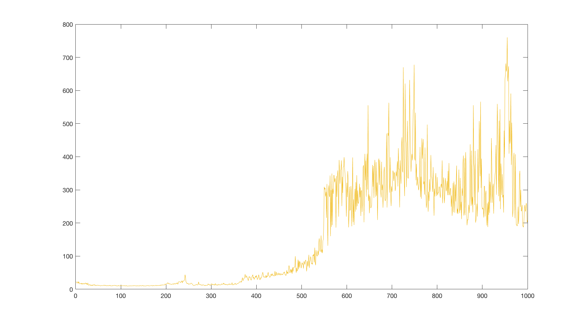
The agent usually learns to hold the pole in straight position after some time, with varying accuracy. To be able to compare results, I ran several thousand episodes with a random policy, which achieved an average reward of 22.6. Then I averaged a reward over 10 runs with our agent, each with 1000 episodes with a limit of 2000 time steps:

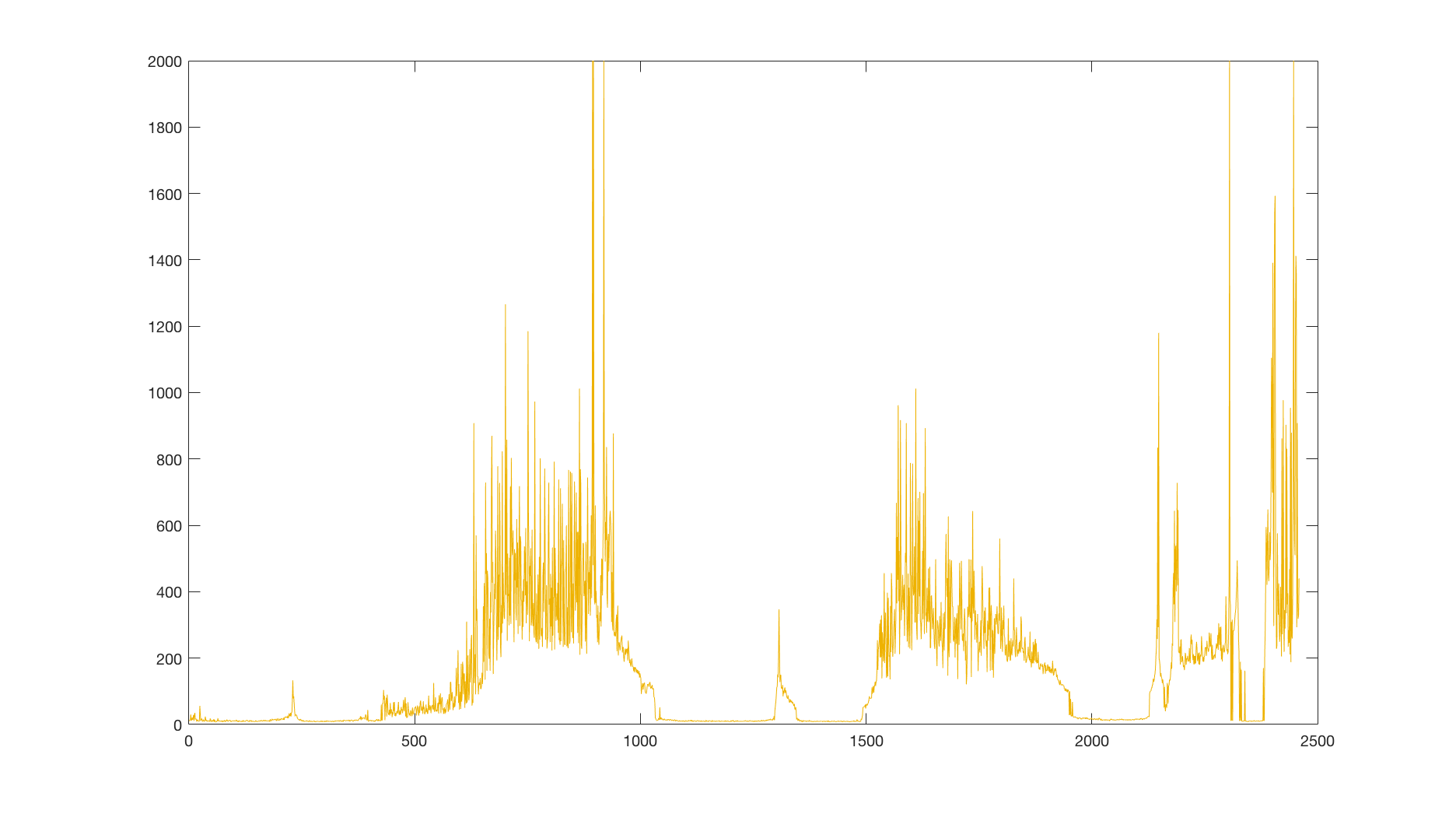
We see that it is well above the average reward of a random policy, so we can conclude that our agent actually learned something. But these results are averaged over multiple runs and the celebrations would be premature. Let’s look at a single run and its reward:

We see that there are several spots where the performance drops suddenly to zero. Clearly, our learning algorithm is unstable. What could be causing these drops and why? Does the network overfit or diverge? Or is it something else? And more importantly, can we mitigate these issues?
As a matter of fact, we can. There are several points in our agent, which we can improve. But before we do that, we have to understand, what the underlaying neural network is doing. In the next section, we will get means to take a meaningful insight into the neural network itself, learn how to display the approximated Q function and use this knowledge to understand what is happening.