This article is part of series Let’s make a DQN.
Introduction
Last time we implemented a Full DQN based agent with target network and reward clipping. In this article we will explore two techniques, which will help our agent to perform better, learn faster and be more stable - Double Learning and Prioritized Experience Replay.
Double Learning
One problem in the DQN algorithm is that the agent tends to overestimate the Q function value, due to the max in the formula used to set targets:
\[Q(s, a) \xrightarrow{} r + \gamma max_a Q(s', a)\]To demonstrate this problem, let’s imagine a following situation. For one particular state there is a set of actions, all of which have the same true Q value. But the estimate is inherently noisy and differs from the true value. Because of the max in the formula, the action with the highest positive error is selected and this value is subsequently propagated further to other states. This leads to positive bias - value overestimation. This severe impact on stability of our learning algorithm1.
A solution to this problem was proposed by Hado van Hasselt (2010)2 and called Double Learning. In this new algorithm, two Q functions - \(Q_1\) and \(Q_2\) - are independently learned. One function is then used to determine the maximizing action and second to estimate its value. Either \(Q_1\) or \(Q_2\) is updated randomly with a formula:
\[Q_1(s, a) \xrightarrow{} r + \gamma Q_2(s', argmax_a Q_1(s', a))\]or
\[Q_2(s, a) \xrightarrow{} r + \gamma Q_1(s', argmax_a Q_2(s', a))\]It was proven that by decoupling the maximizing action from its value in this way, one can indeed eliminate the maximization bias2.
When thinking about implementation into the DQN algorithm, we can leverage the fact that we already have two different networks giving us two different estimates \(Q\) and \(\tilde{Q}\) (target network). Although not really independent, it allows us to change our algorithm in a really simple way.
The original target formula would change to:
\[Q(s, a) \xrightarrow{} r + \gamma \tilde{Q}(s', argmax_a Q(s', a))\]Translated to code, we only need to change one line to get the desired improvements:
t[a] = r + GAMMA * pTarget_[i][ numpy.argmax(p_[i]) ]
The Deep Reinforcement Learning with Double Q-learning1 paper reports that although Double DQN (DDQN) does not always improve performance, it substantially benefits the stability of learning. This improved stability directly translates to ability to learn much complicated tasks.
When testing DDQN on 49 Atari games, it achieved about twice the average score of DQN with the same hyperparameters. With tuned hyperparameters, DDQN achieved almost four time the average score of DQN. Summary of the results is shown in a table in the next section.
Prioritized Experience Replay
One of the possible improvements already acknowledged in the original research2 lays in the way experience is used. When treating all samples the same, we are not using the fact that we can learn more from some transitions than from others. Prioritized Experience Replay3 (PER) is one strategy that tries to leverage this fact by changing the sampling distribution.
The main idea is that we prefer transitions that does not fit well to our current estimate of the Q function, because these are the transitions that we can learn most from. This reflects a simple intuition from our real world - if we encounter a situation that really differs from our expectation, we think about it over and over and change our model until it fits.
We can define an error of a sample S = (s, a, r, s’) as a distance between the Q(s, a) and its target T(S): \(error = |Q(s, a) - T(S)|\)
For DDQN described above, T it would be: \(T(S) = r + \gamma \tilde{Q}(s', argmax_a Q(s', a))\)
We will store this error in the agent’s memory along with every sample and update it with each learning step.
One of the possible approaches to PER is proportional prioritization. The error is first converted to priority using this formula:
\[p = (error + \epsilon)^\alpha\]Epsilon \(\epsilon\) is a small positive constant that ensures that no transition has zero priority. Alpha, \(0 \leq \alpha \leq 1\), controls the difference between high and low error. It determines how much prioritization is used. With \(\alpha = 0\) we would get the uniform case.
Priority is translated to probability of being chosen for replay. A sample i has a probability of being picked during the experience replay determined by a formula:
\[P_i = \frac{p_i}{\sum_k p_k}\]The algorithm is simple - during each learning step we will get a batch of samples with this probability distribution and train our network on it. We only need an effective way of storing these priorities and sampling from them.
Initialization and new transitions
The original paper says that new transitions come without a known error3, but I argue that with definition given above, we can compute it with a simple forward pass as it arrives. It’s also effective, because high value transitions are discovered immediately.
Another thing is the initialization. Remember that before the learning itself, we fill the memory using random agent. But this agent does not use any neural network, so how could we estimate any error? We can use a fact that untrained neural network is likely to return a value around zero for every input. In this case the error formula becomes very simple:
\[error = |Q(s, a) - T(S)| = |Q(s, a) - r - \gamma \tilde{Q}(s', argmax_a Q(s', a))| = | r |\]The error in this case is simply the reward experienced in a given sample. Indeed, the transitions where the agent experienced any reward intuitively seem to be very promising.
Efficient implementation
So how do we store the experience and effectively sample from it?
A naive implementation would be to have all samples in an array sorted according to their priorities. A random number s, \(0 \leq s \leq \sum_k p_k\), would be picked and the array would be walked left to right, summing up a priority of the current element until the sum is exceeded and that element is chosen. This will select a sample with the desired probability distribution.

But this would have a terrible efficiency: O(n log n) for insertion and update and O(n) for sampling.
A first important observation is that we don’t have to actually store the array sorted. Unsorted array would do just as well. Elements with higher priorities are still picked with higher probability.

This releases the need for sorting, improving the algorithm to O(1) for insertion and update.
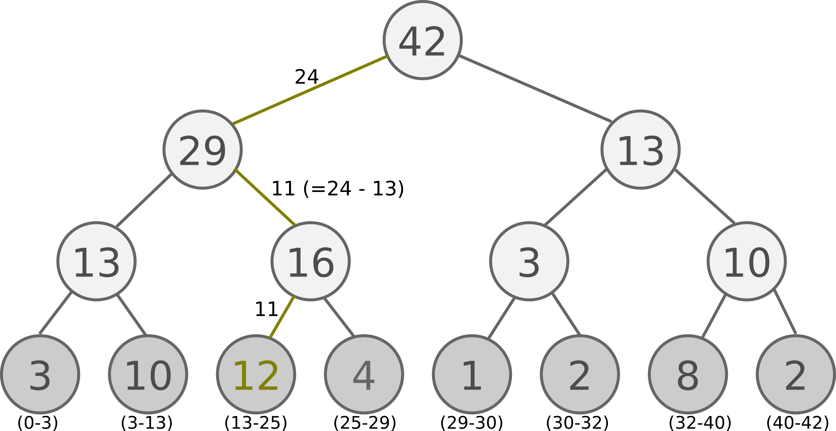
But the O(n) for sampling is still too high. We can further improve our algorithm by using a different data structure. We can store our samples in unsorted sum tree - a binary tree data structure where the parent’s value is the sum of its children. The samples themselves are stored in the leaf nodes.
Update of a leaf node involves propagating a value difference up the tree, obtaining O(log n). Sampling follows the thought process of the array case, but achieves O(log n). For a value s, \(0 \leq s \leq \sum_k p_k\), we use the following algorithm (pseudo code):
def retrieve(n, s):
  if n is leaf_node: return n

  if n.left.val >= s: return retrieve(n.left, s)
  else: return retrieve(n.right, s - n.left.val)
Following picture illustrates sampling from a tree with s = 24:

With this effective implementation we can use large memory sizes, with hundreds of thousands or millions of samples.
For known capacity, this sum tree data structure can be backed by an array. Its reference implementation containing 50 lines of code is available on GitHub.
Results
Tests performed on 49 Atari games showed that PER really translates into faster learning and higher performance3. What’s more, it’s complementary to DDQN.
Following table summarizes the results for 49 Atari games benchmark. Values are taken from Schaul et al. (2015)3 and rescaled. Because the DQN+PER value for proportional PER was not available, the provided value is for similar, but different rank-based PER. For specifics of how these tests were performed, look into the paper3.
| DQN | DQN+PER | DDQN | DDQN+PER |
|---|---|---|---|
| 100% | 291% | 343% | 451% |
Implementation
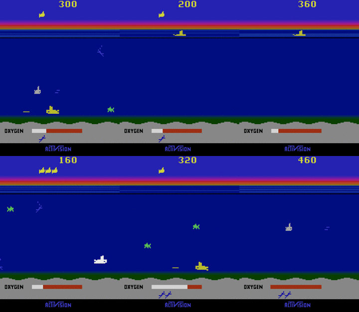
An implementation of DDQN+PER for an Atari game Seaquest is available on GitHub. It’s an improvement over the DQN code presented in last chapter and should be easy to understand.
The DQN architecture from the original paper4 is implemented, although with some differences. In short, the algorithm first rescales the screen to 84x84 pixels and extracts luminance. Then it feeds last two screens as an input to the neural network. This ensures that the algorithm is also aware of a direction of movement of the game elements, something which would not be possible with only a current screen as input. Experience is stored in a sum tree with capacity of 200 000 samples. Neural network uses three convolutional layers and one dense hidden layer with following parameters:
        Convolution2D(32, 8, 8, subsample=(4,4), activation='relu')
        Convolution2D(64, 4, 4, subsample=(2,2), activation='relu')
        Convolution2D(64, 3, 3, activation='relu')
        Dense(output_dim=512, activation='relu')
        Dense(output_dim=actionCount, activation='linear')
These hyperparameters were used:
| Parameter | Value |
|---|---|
| memory capacity | 200000 |
| batch size | 32 |
| γ | 0.99 |
| exploration εmax | 1.00 |
| exploration εmin | 0.10 |
| final exploration frame | 500000 |
| PER α | 0.6 |
| PER ε | 0.01 |
| RMSprop learning rate | 0.00025 |
| target network update frequency | 10000 |
It is possible to run this program on a regular computer, however it is very resource demanding. It takes about 12 GB of RAM and fully utilizes one core of CPU and whole GPU to slowly improve. In my computer it runs around 20 FPS. After about 12 hours, 750 000 steps and 700 episodes, it reached an average reward of 263 (mean reward of a random agent is 87). You can see it in action here:

To get better results, you have to run it for at least tens of millions of steps. The following graph shows that the improvement is indeed very slow:

Conclusion
We addressed Double Learning and Prioritized Experience Replay techniques that both substantially improve the DQN algorithm and can be used together to make a state-of-the-art algorithm on the Atari benchmark (at least as of 18 Nov 2015 - the day Prioritized Experience Replay3 article was published).
This articles finishes the Let’s make a DQN series. It was meant as a simplified tutorial for those who don’t want to read whole research articles but still want to understand what DQN is and what it does. I also hope that it sparkled your interest in this interesting direction of AI and that you will want to learn even more now.
I hope you enjoyed these articles at least as me writing them and that you learned something. If you have any questions or have anything to add, please feel free to leave a comment or contact me at author@jaromiru.com.
References
-
Hado van Hasselt, Arthur Guez, David Silver - Deep Reinforcement Learning with Double Q-learning, arXiv:1509.06461, 2016 ↩ ↩2
-
Hado van Hasselt - Double Q-learning, Advances in Neural Information Processing Systems, 2010 ↩ ↩2 ↩3
-
Schaul et al. - Prioritized Experience Replay, arXiv:1511.05952, 2015 ↩ ↩2 ↩3 ↩4 ↩5 ↩6
-
Mnih et al. - Human-level control through deep reinforcement learning, Nature 518, 2015 ↩