This article is part of series Let’s make a DQN.
Introduction
Last time we saw that our Q-learning can be unstable. In this article we will cover some methods that will help us to understand what is going on inside the network.
The code for this article can be found at github.
Problem
For this article we will choose a different environment - MountainCar-v0, which looks like this:
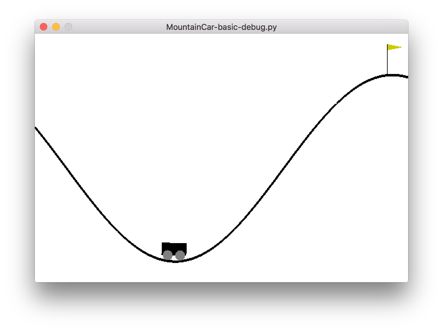
The goal is to get a car to a flag, which can be seen on the right. The car has to get from the valley, represented by the black line, by accumulating enough momentum. The task is always the same, although the starting position of the car changes with each episode.
The state is represented by only two variables - position and speed of the car. For every time step, the agent receives a reward of -1, until it reaches its goal. There are two actions - push the car left or right.
In MountainCar environment, the agent is continuously penalized and it has to finish the episode as quickly as possible. This is in contrast with the CartPole environment, where the agent accumulated positive reward and tried to prolong the episode for as long as possible.
The simplicity of state space, which is only two dimensional, will allow us to represent it in a human readable way.
Implementation
The coded made in the last article is robust enough to cover also this problem, with only slight changes. However, some improvements and additions were made.
Initialization with random agent
In the beginning of the learning, the agent has an empty memory and also does not know yet what actions to take. We can assume, that a random policy would do the same job in choosing actions, but at much higher rate. Therefore we can simply fill the memory of the agent before the start of the learning itself with a random policy.
Test made with random policy showed that it finishes the episode approximately after 14 000 steps. With memory capacity of 100 000 steps, the agent starts its learning with about 7 episodes of data. This will typically speed up the learning process.
Action reduction
The original OpenGym environment has three actions - push left, do-nothing and ush right. The do-nothing action is not needed for solving the problem and will only make the learning more difficult. The point of this article is to demonstrate debugging techniques and this added complexity is not needed. Therefore the actions were remapped so that the do-nothing action is not used.
Hyperparameters
All of the parameters stay the same, except for εmin, which was raised to 0.1.
Normalization
Tests showed that normalizing states doesn’t give any substantial advantage in this problem. However, if we normalize every state variable into [-1 1] region, it allows us to display them in a simple way later.
Debugging
Q function visualization
The network inside the agent is learning a Q function. Let’s recall what this function means. It is an estimate of a discounted total reward the agent would achieve starting in position s and taking action a. The true function also satisfies a property:
\[Q(s, a) = r + \gamma \max_a Q(s', a)\]So, it is desirable that we understand how this function looks and what it means.
Right from the start we can estimate its range. In this problem the agent always receives a reward of -1 whatever action it takes. At the end of the episode the transition goes straight to the terminal state, for which the Q function is known:
\[Q(s, a) = r\]Reward r is in this case -1 and at the same time it is the upper bound. In all other non-terminal states it will be lesser than -1.
If we have a minimal sequence of actions leading to a terminal state, starting at a state s and taking a first action a, the value of the Q(s, a) would be:
\[Q = r + \gamma r + \gamma^2 r + ... = r\frac{1-\gamma^n}{1-\gamma}\]For an infinite sequence, this gives us the lower bound:
\[Q = -\frac{1}{1-0.99} = -100\]The range of the Q function for all states and actions is therefore:
\[-100 \leq Q(s, a) \leq -1\]We can now pick pick several points in the Q function and track their values, as the learning progresses. Points of particular interest are at the start and at just before the end of an episode.
By using a trained agent I generated an episode which lasted for 91 steps. Let’s pick these four particular states from it:
    [-0.15955113,  0.        ]  # s_start

    [ 0.83600049,  0.27574312]  # s'' -> s'
    [ 0.85796947,  0.28245832]  # s' -> s
    [ 0.88062271,  0.29125591]  # s -> terminal
The correct action in the last three states is to push right, so let’s pick this action and track the Q function at these points. We can do this by simply by calling brain.predict(states).
The expected values at s is -1 and with each step backwards it decreases. We can compute an approximate value for sstart using the formula above to be about -60. The expected values are summarized below:
  Q(s, right)     = -1
  Q(s', right)      = -1.99
  Q(s'', right)     = -2.97
  Q(s_start, right) ~ -60
The following graph shows a single run of the algorithm, with the values of the estimated Q function tracked every 1000 steps. Each line correspond to one point in the Q function:
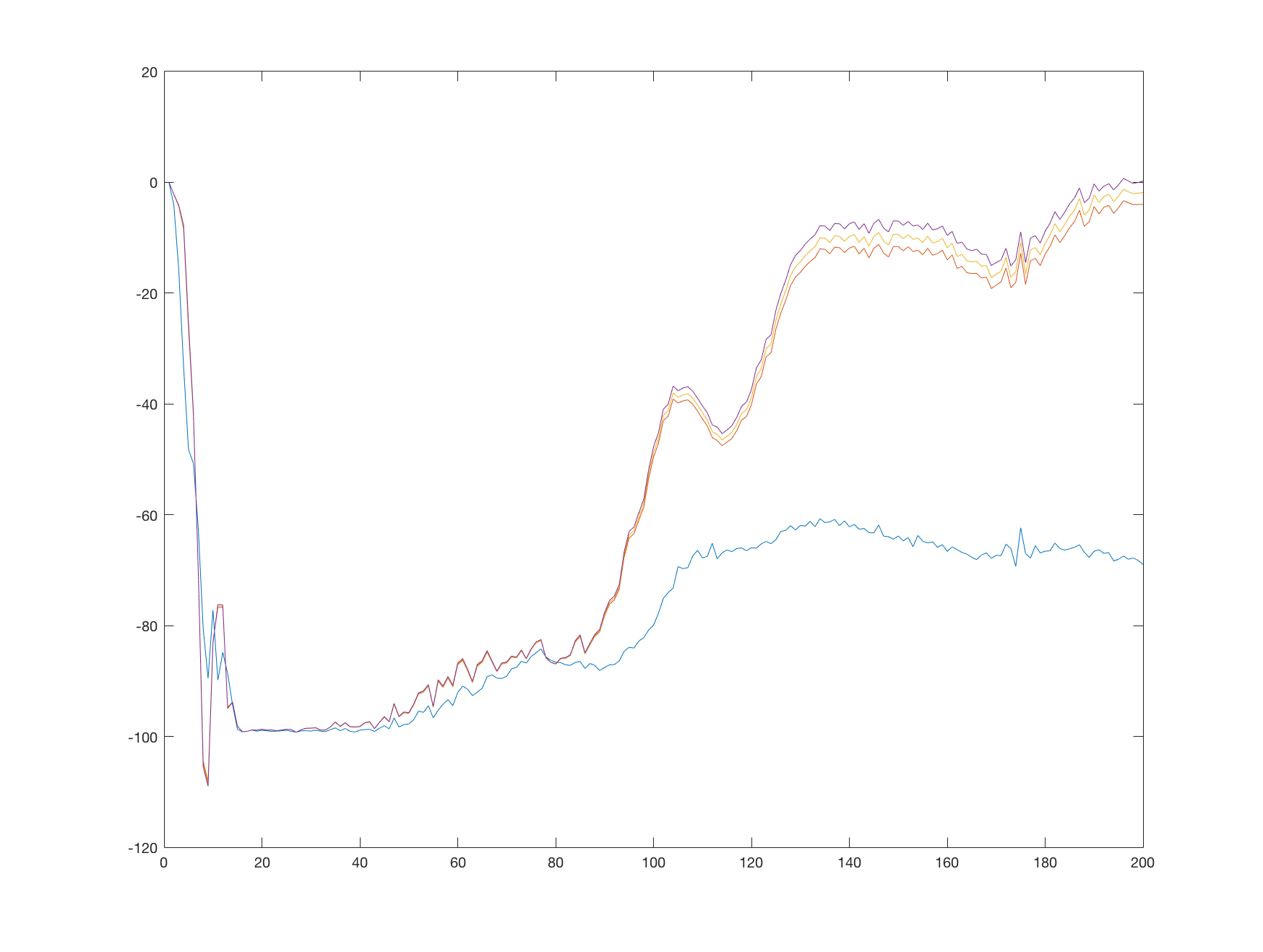
We see that the values start at 0, quickly descending to the minimum of 100. When the learning stabilizes, the terminal transitions start to influence the estimated Q function and this information starts to propagate to other states. After 200 000 steps the Q function values at the tracked points resembles our hand-made estimates. Which line correspond to which point is clear when compared to our estimates.
When we look at the learning after 1 500 000 steps, the chart looks like this:
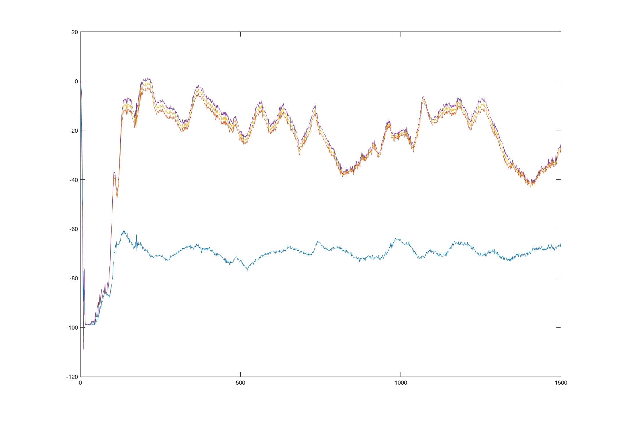
We see that the values oscillate, but keep their relative distance and always tend to return to their true values. This might happen due to several reasons, which we will discuss later.
Value function visualization
Similar to Q function is a value function V(s). It’s defined as a total discounted reward starting at state s and following some policy afterwards. With a greedy policy we can write the value function in terms of the Q function:
\[V(s) = \max_a Q(s, a)\]Because a state in our problem is only two dimensional, it can be visualized as a 2D color map. To more augment this view, we can add another map, showing actions with highest value at a particular point.
We can extract these values from our network by simple forward pass for each point in our state space, with some resolution. Because we normalized our states to be in [-1 1] range, the corresponding states falls to a [-1 1 -1 1] rectangle.
Using a neural network with one hidden layer consisting of 64 neurons, we can generate the following image. It shows both of our maps.
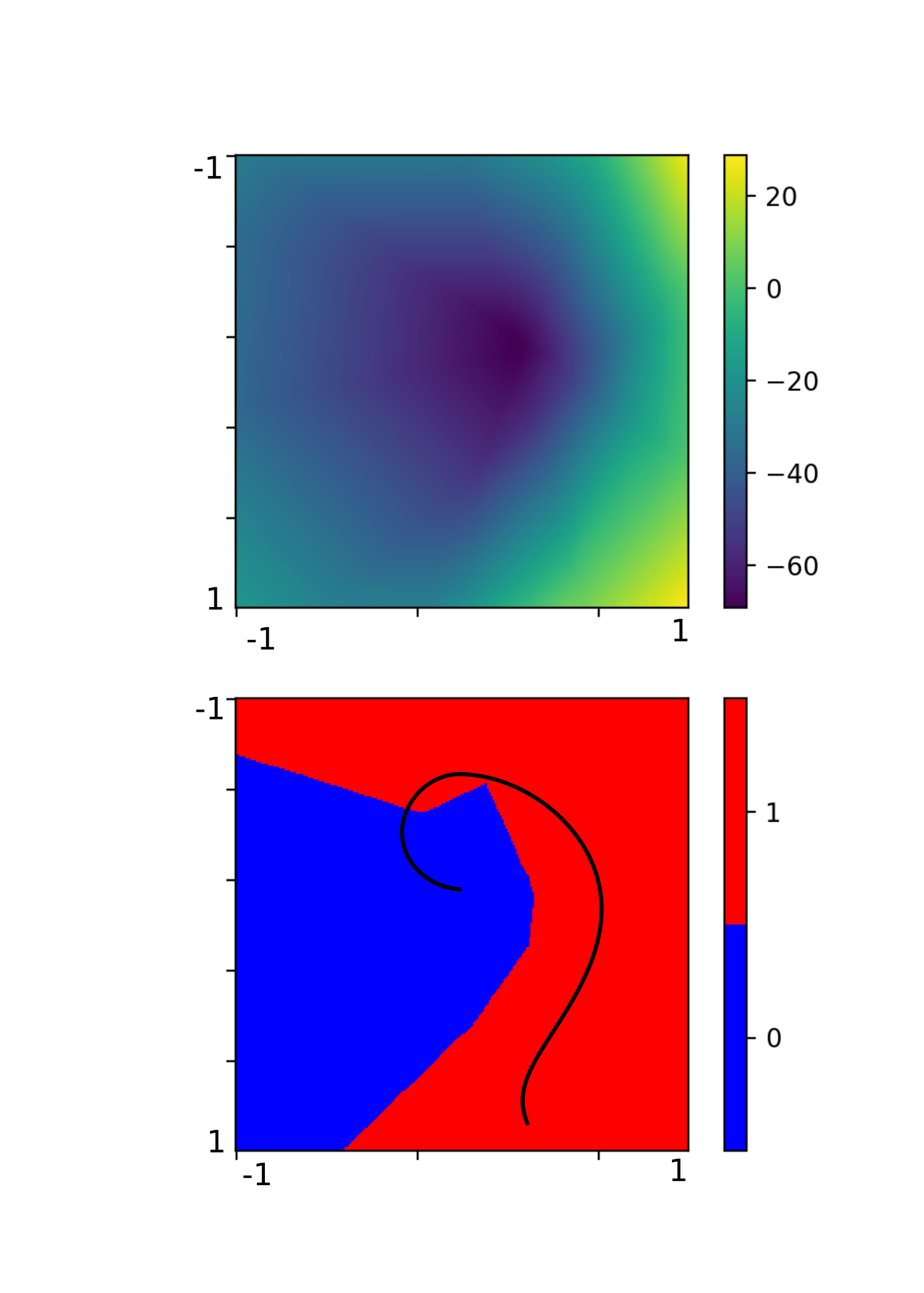
The upper part is a color map of the value function and the bottom part shows areas where the Q function is higher for left (0 or blue) or right (1 or red) action. The vertical axis corresponds to car position and the horizontal axis corresponds to car velocity. The black line shows a trajectory the agent took in a single sample episode.
From the bottom part we can see that the agent did a very good job in generalizing what action to take in which state. The distinction between the two actions is very clear and seems reasonable. The right part of the map corresponds to high speed towards the right of the screen. In these cases the agent always chooses to push more right, because it will likely hit the goal.
Let’s recall how the environment looks like:

The top part in the map corresponds to position on the left slope, from which the agent can gain enough momentum to overcome the slope on the right, reaching the goal. Therefore the agent chooses the push right action.
The blue area corresponds to points where the agent has to get on the left slope first, by choosing the push left action.
The value function itself seems to be correct - the lowest values are in the center, where the agent has no momentum and will likely spend most time getting it, with it’s value raising towards the right and bottom part, corresponding to high right velocity, and position closer to the goal.
However, the right top and bottom corners greater than -1 and are out of the predicted range. This is probably because these states (on the slope left and high right velocity and on the slope right and high right velocity) are never encountered during the learning. Most likely it’s not a problem.
Comparing to high order network
Looking at the value function itself, it seems to be a little fuzzy. It’s unprobable that the true value function is that smooth in all directions. A more sophisticated network could possibly learn a better approximation. Let’s use a network with two hidden layers, each consisting of 256 neurons. First, let’s look at the Q function values graph at the same points as before:
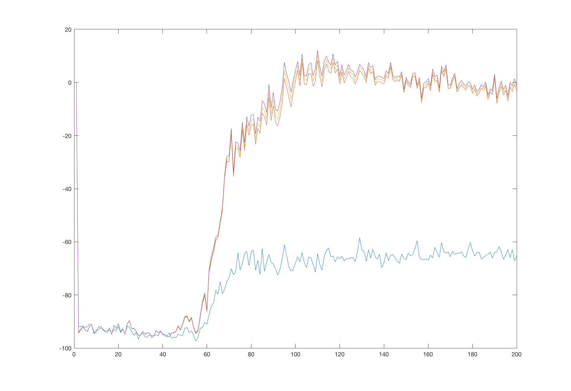
Interestingly, the network converged to the true values quicker than its weaker version. But what is more surprising is that it managed to hold its values around the true values:
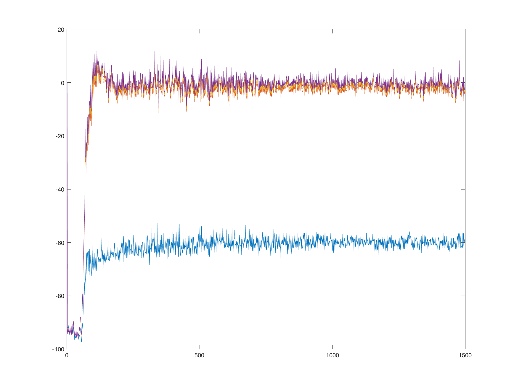
Counterintuitively, the higher order network seems to be more stable. Let’s look at the value function visualization:
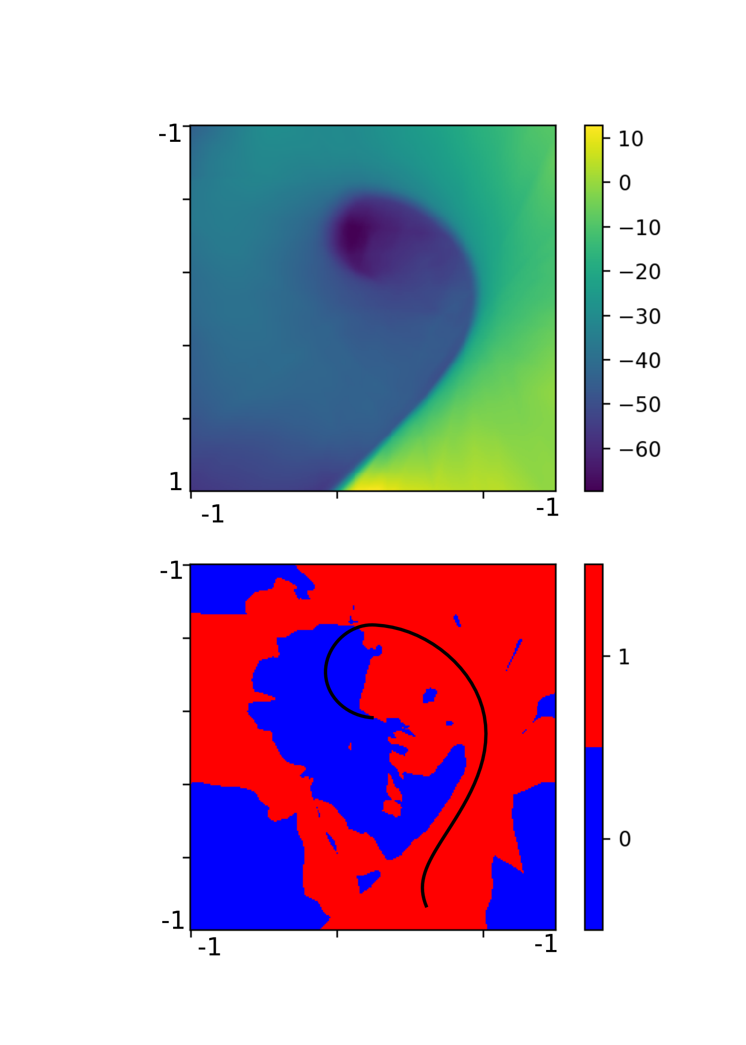
At a first glance we can see that the approximation of the value function is much better. However, the action map is a little overcomplicated.
For example, the blue spots on the right, although probably never met in the simulation, are most likely to be incorrect. It seems that our network overfit the training samples and failed to generalize properly beyond them. This also explains the higher speed of convergence and sustained values - the network with many more parameters can accommodate more of specific values easily, but cannot generalize well for values nearby.
We can now conclude that the previous oscillations in the simpler network might have been caused by its insufficient capability to incorporate all the knowledge. Different training samples pull the network in different directions and it unable to satisfy all of them, leading to oscillations.
CartPole revisited
Let’s go back and look at the previous problem - the CartPole environment. We noticed, that its performance suffered several drops, but were unable to say why. With our current knowledge we can plot a joint graph of the reward and a point at the Q function. The point is chosen to be around a sustainable upward position, therefore the agent could theoretically hold the pole upwards indefinitely starting at this state. The true value of the Q function at this state can be computed as \(Q = \frac{1}{1-0.99} = 100\).
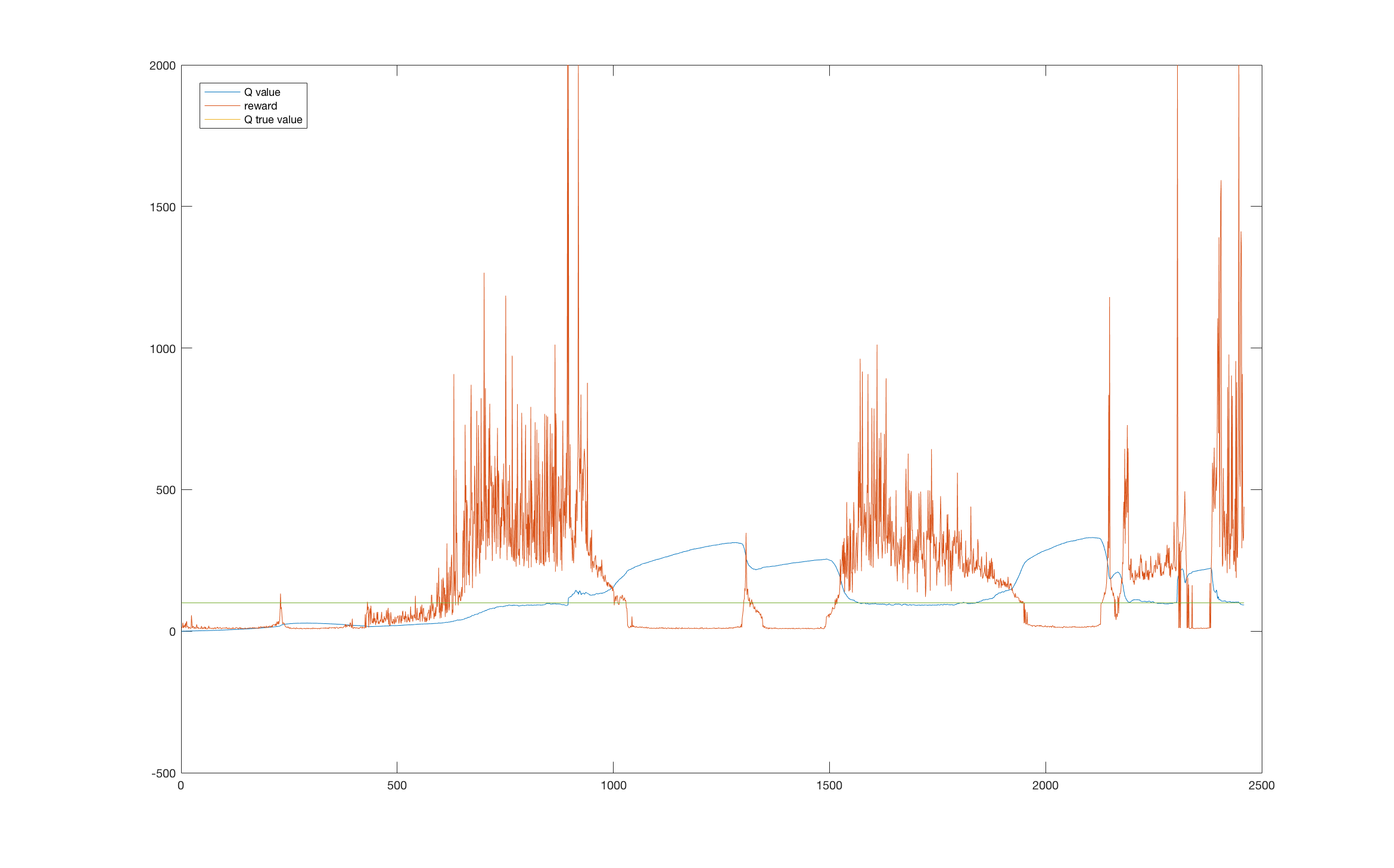
Looking at the graph we can see that the performance drops highly correspond to areas where the value function was overestimated. This could be caused by maximization bias and insufficient exploration.
Reasons of instability
We have identified a few reasons for Q-learning instability. We will now present them briefly, along with other not discussed here and leave thorough discussion to another articles.
Unappropriate network size
We saw that a small network may fail to approximate the Q function properly, whereas a large network can lead to overfitting. Careful network tuning of a network size along with other hyper-parameters can help.
Moving targets
Target depends on the current network estimates, which means that the target for learning moves with each training step. Before the network has a chance to converge to the desired values, the target changes, resulting in possible oscillation or divergence. Solution is to use a fixed target values, which are regularly updated1.
Maximization bias
Due to the max in the formula for setting targets, the network suffers from maximization bias, possibly leading to overestimation of the Q function’s value and poor performance. Double learning can help2.
Outliers with high weight
When a training is performed on a sample which does not correspond to current estimates, it can change the network’s weights substantially, because of the high loss value in MSE loss function, leading to poor performance. The solution is to use a loss clipping1 or a Hubert loss function.
Biased data in memory
If the memory contain only some set of data, the training on this data can eventually change the learned values for important states, leading to poor performance or oscillations. During learning, the agent chooses actions according to its current policy, filling its memory with biased data. Enough exploration can help.
Possible improvements
There are also few ideas how to improve the Q-learning itself.
Prioritized experience replay
Randomly sampling form a memory is not very efficient. Using a more sophisticated sampling strategy can speed up the learning process3.
Utilizing known truth
Some values of the Q function are known exactly. These are those at the end of the episode, leading to the terminal state. Their value is exactly \(Q(s, a) = r\). The idea is to use these values as anchors, possibly with higher weight in the learning step, which the network can hold to.
Conclusion
We saw two methods that help us to analyze the Q-learning process. We can display the estimated Q function in known points in a form of graph and we can display a map of a value function in a color map, along with a action map. We also saw what are some of the reasons of Q-learning instability and possible improvements. In the next article we will make a much more stable solution based on a full DQN network.
References
-
Mnih et al. - Human-level control through deep reinforcement learning, Nature 518, 2015 ↩ ↩2
-
Hasselt et al. - Deep Reinforcement Learning with Double Q-learning, arXiv:1509.06461, 2015 ↩
-
Schaul et al. - Prioritized Experience Replay, arXiv:1511.05952, 2015 ↩