Let’s make a DQN: Full DQN

Introduction

Up until now we implemented a simple Q-network based agent, which suffered from instability issues. In this article we will address these problems with two techniques - target network and error clipping. After implementing these, we will have a fully fledged DQN, as specified by the original paper¹.

Target Network

During training of our algorithm we set targets for gradient descend as:

We see that the target depends on the current network. A neural network works as a whole, and so each update to a point in the Q function also influences whole area around that point. And the points of Q(s, a) and Q(s’, a) are very close together, because each sample describes a transition from s to s’. This leads to a problem that with each update, the target is likely to shift. As a cat chasing its own tale, the network sets itself its targets and follows them. As you can imagine, this can lead to instabilities, oscillations or divergence.

To overcome this problem, researches proposed to use a separate target network for setting the targets. This network is a mere copy of the previous network, but frozen in time. It provides stable \(\tilde{Q}\) values and allows the algorithm to converge to the specified target:

After severals steps, the target network is updated, just by copying the weights from the current network. To be effective, the interval between updates has to be large enough to leave enough time for the original network to converge.

A drawback is that it substantially slows down the learning process. Any change in the Q function is propagated only after the target network update. The intervals between updated are usually in order of thousands of steps, so this can really slow things down.

On the graph below we can see an effect of a target network in MountainCar problem. The values are plotted every 1000 steps and target network was updated every 10000 steps. We can see the stair-shaped line, where the network converged to provided target values. Each drop corresponds to an update of the target network.

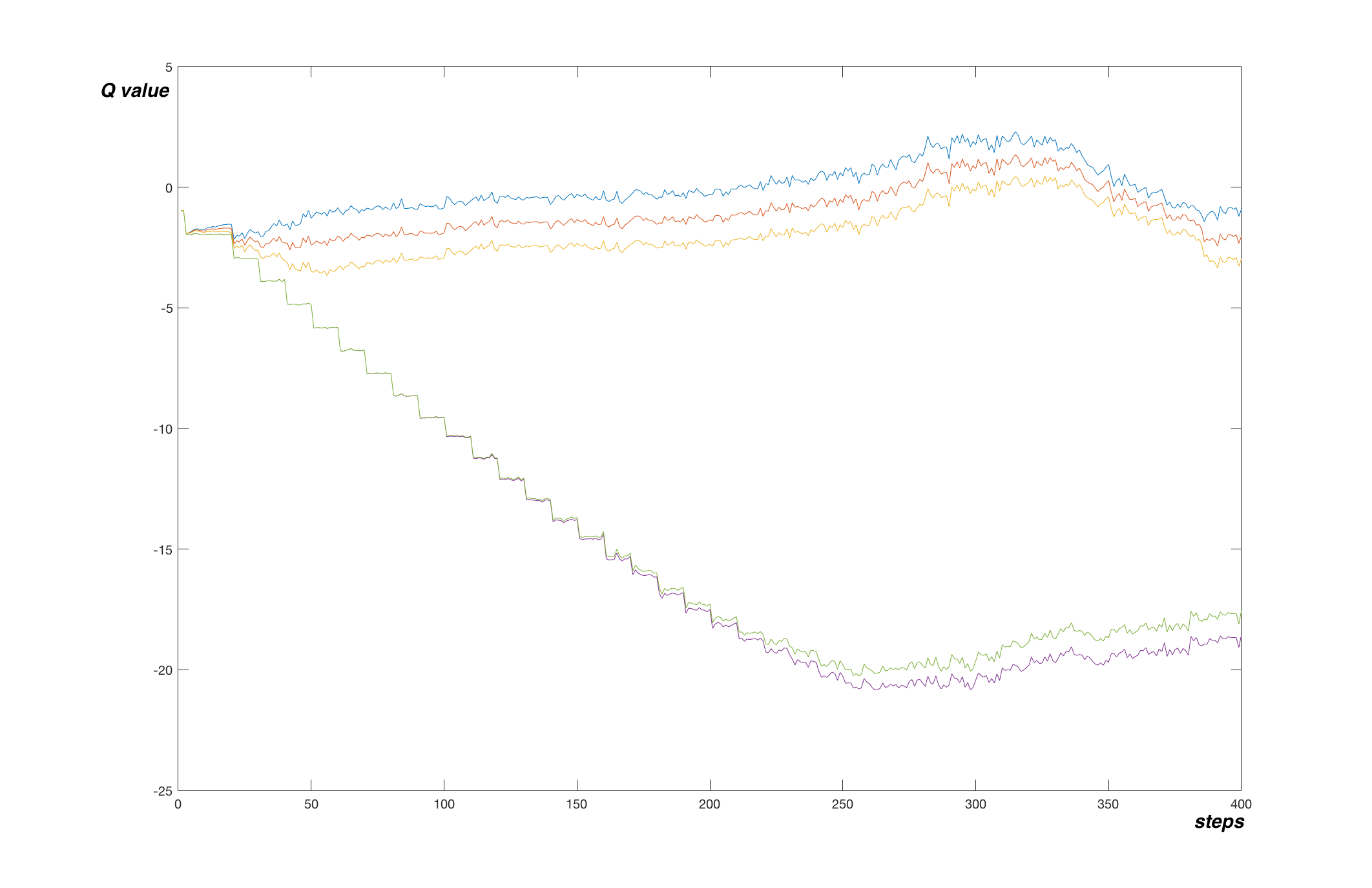
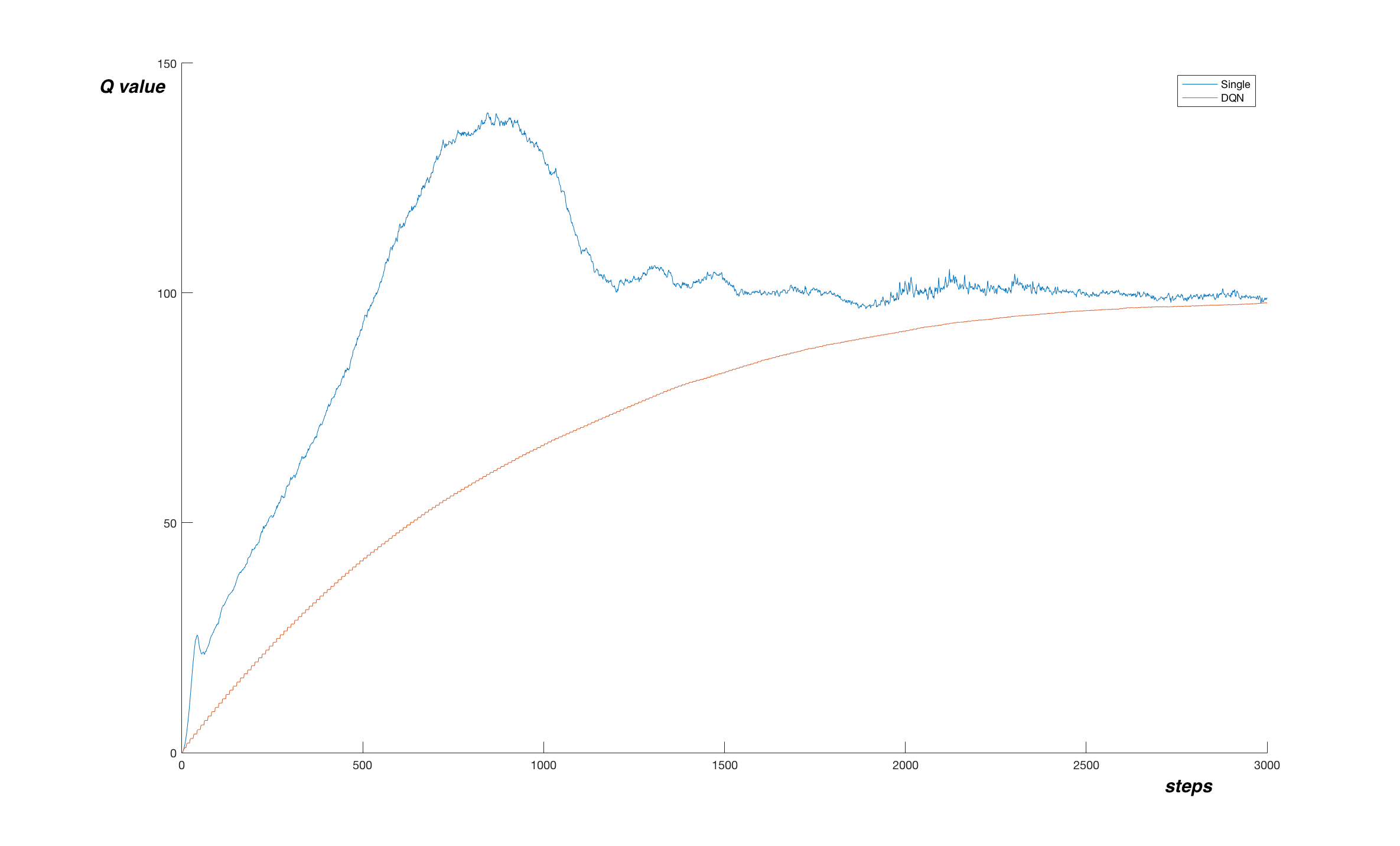
The network more or less converged to true values after 250 000 steps. Let’s look at a graph of a simple Q-network from last article (note that tracked Q function points are different):

Here the algorithm converged faster, after only 100 000 steps. But the shape of the graph is very different. In the simple Q-network variant, the network went fast to the minimum of -100 and started picking the final transitions to reach true values after a while. The algorithm with target network on the other hand quickly anchored the final transitions to their true values and slowly propagated this true value further to the network.

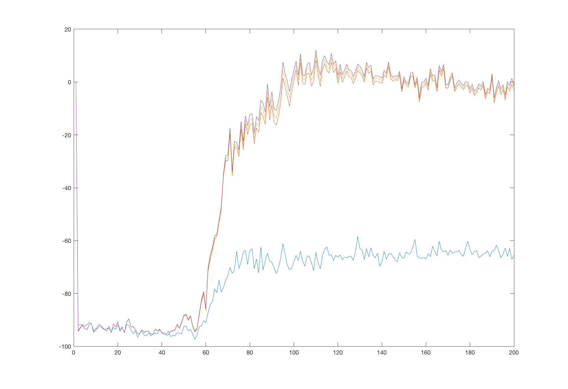
Another direct comparison can be done on the CartPole problem, where the differences are clear:

The version with target network smoothly aim for the true value whereas the simple Q-network shows some oscillations and difficulties.

Although sacrificing speed of learning, this added stability allows the algorithm to learn correct behaviour in much complicated environments, such as those described in the original paper¹ - playing Atari games receiving only visual input.

Error clipping

In the gradient descend algorithm, usually Mean Squared Error (MSE) loss function is used. It is defined as:

where \(t_i\) and \(y_i\) are targets and predicted values in i-th sample. For each sample there is the error term \((t - y)^2\). This error value can be huge for a sample which is not in alignment with the current network prediction. The loss function is directly used in the backward propagation algorithm and large errors cause large changes to the network.

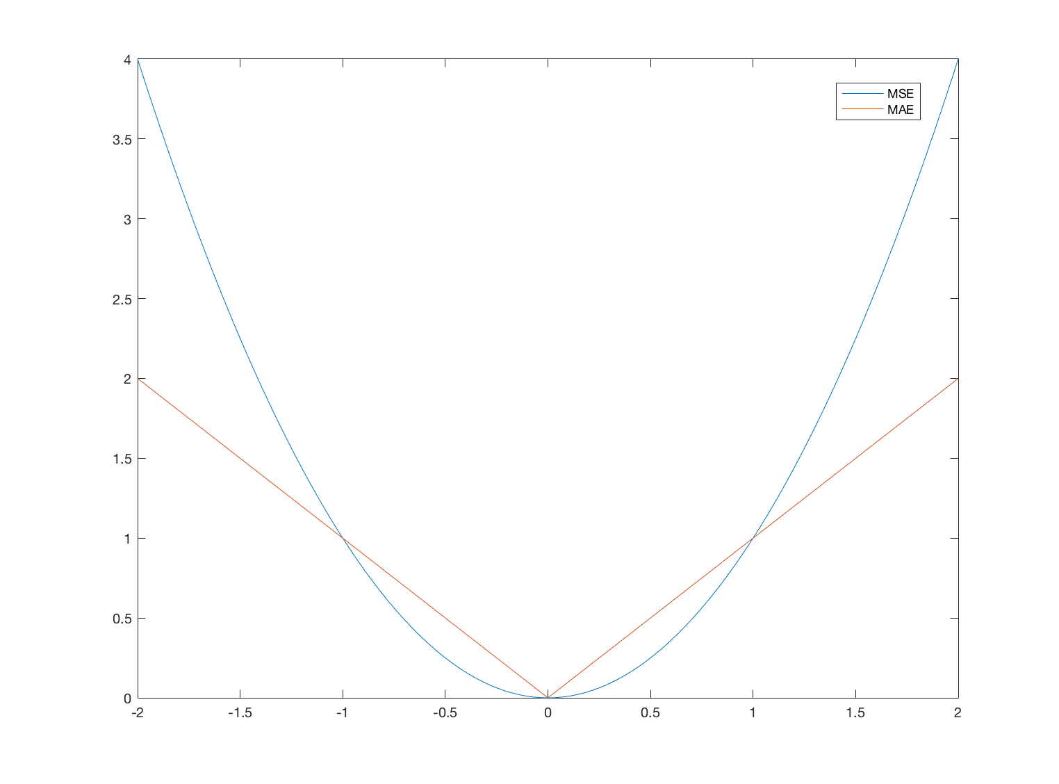
By choosing a different loss function, we can smooth these changes. In the original paper¹, clipping of the derivative of MSE to [-1 1] is proposed. This effectively means that MSE is used for errors in the [-1 1] region and Mean Absolute Error (MAE) outside. MAE is defined as:

The differences between the two functions are shown in the following image:

Note that based on recent insight (see discussion), the pseudo-huber loss function described below is incorrect to use. Use the original Huber function with reward clipping or MSE.

There’s actually a different way of describing such a loss function, in a single quotation. It’s called Pseudo-Huber loss and is defined as

and looks like this:

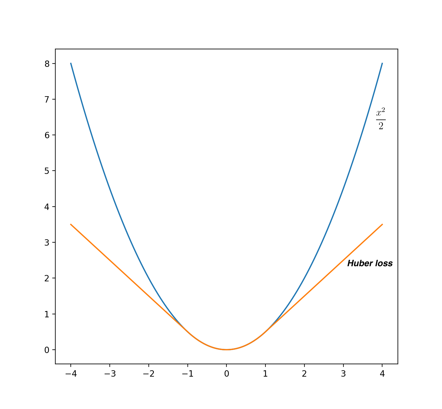
It behaves as \(\frac{x^2}{2}\) in [-1 1] region and as \(|x| - \frac{1}{2}\) outside, which is almost the same as the error clipping described above. This loss function is prefect for our purposes - it is fully differentiable and it’s one line of code.
However, the error clipping technique have its drawbacks. It it important to realize that in the back-propagation algorithm, its derivative is actually used. Outside [-1 1] region, the derivative is either -1 or 1 and therefore all errors outside this region will get fixed slowly and at the same constant rate. In some settings this can cause problems. For example in the CartPole environment, the combination of simple Q-network and Huber loss actually systematically caused the network to diverge.

Implementation

You can download a demonstration of DQN on the CartPole problem from github.

The only changes against the old versions are that the Brain class now contains two networks model and model_ and we use the target network in the replay() function to get the targets. Also, the initialization with random agent is now used.

Let’s look at the performance. In the following graph, you can see smoothed reward, along with the estimated Q value in one point. Values were plotted every 1000 steps.

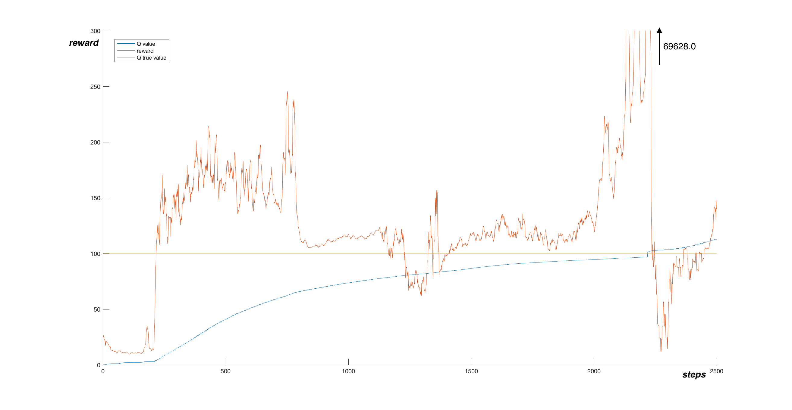
We see that the Q function estimate is much more stable than in the simple Q-learning case. The reward tend to be stable too, but at around step 2 200 000, the reward reached an astronomical value of 69628.0, after which the performance dropped suddenly. I assume this is caused by limited memory and experience bias. During this long episode, almost whole memory was filled with highly biased experience, because the agent was holding the pole upright, never experiencing any other state. The gradient descend optimized the network using only this experience and while doing so destroyed the previously learned Q function as a whole.

Conclusion

This article explained the concepts of target network and error clipping, which together with Q-learning form full DQN. We saw how these concepts make learning more stable and offered a reference implementation.

Next time we will look into further improvements, by using Double learning and Prioritized Experience Replay.

References